Overview
R-itable estimates narrow-sense heritability (h²) for quantitative traits in family cohort studies using a profile-likelihood variance-components approach, without requiring SOLAR Eclipse or any proprietary software.
The three main steps are:
- Build the additive genetic relationship matrix (GRM) from a pedigree.
- Estimate heritability for one trait with
herit_vc(). - Scale to many traits with
herit_batch(), then visualise withplot_forest().
For twin cohorts specifically – monozygotic relatedness,
household/shared- environment effects, and bivariate
genetic/environmental correlations between two traits – see
vignette("twin-cohorts") instead/in addition.
1. Build the GRM
build_grm() takes a pedigree data frame and returns an
additive genetic relationship matrix (GRM, also written
A). The GRM encodes how much genetic material any two
individuals share due to common ancestry, and is the cornerstone of the
variance-components model.
The pedigree needs four columns:
| Column | Content |
|---|---|
id |
Individual ID |
pat |
Father’s ID (0 or NA for founders) |
mom |
Mother’s ID (0 or NA for founders) |
sex |
1 = male, 2 = female |
Importantly, the pedigree should contain everyone —
both the study subjects you want to analyse and their
parents/grandparents (founders), even if the founders have no phenotype
data. Including founders lets kinship2 trace shared
ancestry correctly.
In the example below, IDs 1–4 are two unrelated founder couples. IDs 5–6 are offspring of couple 1×2, and IDs 7–8 are offspring of couple 3×4. The study subjects are IDs 5–8.
ped <- data.frame(
  id  = 1:8,
  pat = c(0, 0, 0, 0, 1, 1, 3, 3),  # founders have pat = 0
  mom = c(0, 0, 0, 0, 2, 2, 4, 4),  # founders have mom = 0
  sex = c(1, 2, 1, 2, 1, 2, 1, 2)
)

A <- build_grm(ped, study_ids = 5:8)
round(A, 3)
#>     5   6   7   8
#> 5 1.0 0.5 0.0 0.0
#> 6 0.5 1.0 0.0 0.0
#> 7 0.0 0.0 1.0 0.5
#> 8 0.0 0.0 0.5 1.0
Reading the matrix:
- Diagonal = 1 for non-inbred individuals (each person shares 100% of their genome with themselves).
- 5 & 6 share 0.5 — they are full siblings (same parents 1×2), so they share on average half their segregating alleles.
- 7 & 8 share 0.5 — full siblings of couple 3×4, same logic.
- 5 & 7 share 0 — their parents come from entirely different founders, so they are genetically unrelated in this pedigree.
This block-diagonal pattern is typical of a study with multiple independent families. In a real cohort the pedigree is often more complex (multi-generation, distant relatives), but the interpretation is the same: larger off-diagonal values mean more shared ancestry.
2. Estimate heritability for a single trait
set.seed(42)

# Simulate some phenotype data for the study subjects
dat <- data.frame(
  IID     = 5:8,
  age     = c(35, 38, 40, 44),
  sex_num = c(1, 2, 1, 2),
  bmi     = c(24.1, 27.3, 22.8, 29.5)
)

# Unadjusted model
res_unadj <- herit_vc("bmi", grm = A, data = dat, min_n = 3)
#> ✔ bmi_unadj  n=4  h2=0.001 [0,1]  p=0.5

# Adjusted model (age + sex)
res_adj <- herit_vc("bmi", grm = A, data = dat,
                    covs  = c("age", "sex_num"),
                    label = "bmi_adj",
                    min_n = 3)
#> ✔ bmi_adj  n=4  h2=0.001 [NA,NA]  p=0.5

str(res_unadj)
#> List of 12
#>  $ label         : chr "bmi_unadj"
#>  $ trait         : chr "bmi"
#>  $ covariates    : chr ""
#>  $ n             : int 4
#>  $ h2            : num 0.001
#>  $ se            : num 44.7
#>  $ ci_lo         : num 0
#>  $ ci_hi         : num 1
#>  $ pval          : num 0.5
#>  $ var_covariates: num NA
#>  $ sigma2_a      : num 0.00039
#>  $ sigma2_e      : num 0.386
The returned list contains:
| Field | Description |
|---|---|
h2 |
MLE narrow-sense heritability |
se |
SE from profile-LL curvature |
ci_lo, ci_hi
|
95% profile-likelihood CI |
pval |
One-sided LRT p-value (boundary-corrected) |
var_covariates |
Variance explained by fixed-effect covariates (R²); NA
for unadjusted models |
sigma2_a |
Additive genetic variance (σ²_g) |
sigma2_e |
Residual environmental variance (σ²_e) |
3. Batch estimation
For real analyses you will typically run many traits across several
covariate models. herit_batch() handles this and returns a
tidy data frame.
# Add a second trait
dat$hdl <- c(55.0, 60.2, 48.3, 72.1)

covs_list <- list(
  unadj = NULL,
  cov1  = c("age", "sex_num")
)

res <- herit_batch(
  traits    = c("bmi", "hdl"),
  grm       = A,
  data      = dat,
  covs_list = covs_list,
  min_n     = 3,
  .progress = FALSE
)

res
#>       label trait  covariates n    h2      se ci_lo ci_hi pval var_covariates
#> 1 bmi_unadj   bmi             4 0.001 44.7184     0     1  0.5             NA
#> 2 hdl_unadj   hdl             4 0.001 44.7184     0     1  0.5             NA
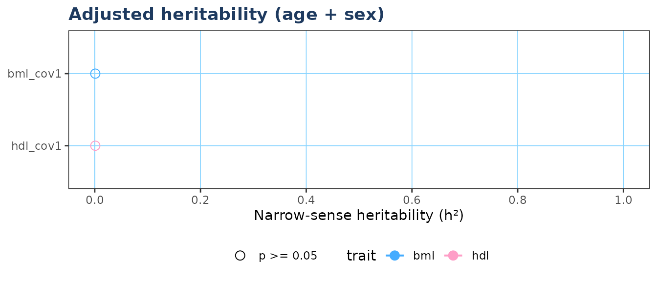
#> 3  bmi_cov1   bmi age+sex_num 4 0.001      NA    NA    NA  0.5         0.7778
#> 4  hdl_cov1   hdl age+sex_num 4 0.001      NA    NA    NA  0.5         0.7778
#>   sigma2_a sigma2_e
#> 1  0.00039  0.38606
#> 2  0.00039  0.38606
#> 3  0.00009  0.08576
#> 4  0.00009  0.08576
4. Forest plot
if (requireNamespace("ggplot2", quietly = TRUE)) {
  plot_forest(res,
              model_filter  = "cov1",
              colour_by     = "trait",
              title         = "Adjusted heritability (age + sex)")
}
5. Colour palette
Ritable_colours is exported for consistent figure
styling across your analysis. It contains the four brand colours used in
plot_forest() by default:
Ritable_colours
#>      pink      blue       sky     cream
#> "#FE9EC7" "#44ACFF" "#89D4FF" "#F9F6C4"
You can use them directly in ggplot2 calls:
ggplot2::scale_colour_manual(values = Ritable_colours[c("blue", "pink")])6. Realistic workflow
Here we simulate a small multi-family cohort — 80 nuclear families, 2 parents + 3 offspring each — with three phenotypes that have different true h² values. This mirrors what you would do with real pedigree and phenotype CSV files.
library(Ritable)

# ---- 1. Simulate pedigree ---------------------------------------------------
set.seed(2026)
n_fam <- 80

ped <- do.call(rbind, lapply(seq_len(n_fam), function(f) {
  base <- (f - 1L) * 5L
  data.frame(
    id  = base + 1:5,
    pat = c(0L, 0L, base + 1L, base + 1L, base + 1L),
    mom = c(0L, 0L, base + 2L, base + 2L, base + 2L),
    sex = c(1L, 2L, sample(1:2, 3, replace = TRUE))
  )
}))

# ---- 2. Simulate phenotypes for offspring -----------------------------------
# Three traits with approximate h2: bmi ~0.6, sbp ~0.35, hdl ~0.5
simulate_trait <- function(ped, n_fam, h2, seed) {
  set.seed(seed)
  genetic  <- rep(rnorm(n_fam, 0, sqrt(h2)),       each = 5)
  residual <- rnorm(nrow(ped),          0, sqrt(1 - h2))
  genetic + residual
}

pheno_all <- data.frame(
  bmi = simulate_trait(ped, n_fam, h2 = 0.60, seed = 1),
  sbp = simulate_trait(ped, n_fam, h2 = 0.35, seed = 2),
  hdl = simulate_trait(ped, n_fam, h2 = 0.50, seed = 3)
)

off_rows <- ped$pat != 0L
dat <- data.frame(
  IID     = ped$id[off_rows],
  age     = round(runif(sum(off_rows), 20, 75)),
  sex_num = ped$sex[off_rows],
  bmi     = pheno_all$bmi[off_rows],
  sbp     = pheno_all$sbp[off_rows],
  hdl     = pheno_all$hdl[off_rows]
)
dat$age2 <- dat$age^2

# ---- 3. Build GRM once — reuse for all models -------------------------------
A <- build_grm(ped, study_ids = dat$IID)

# ---- 4. Define covariate models ---------------------------------------------
covs_list <- list(
  unadj = NULL,
  cov1  = c("age", "sex_num"),
  cov2  = c("age", "sex_num", "age2")
)

# ---- 5. Batch estimation ----------------------------------------------------
res <- herit_batch(
  traits    = c("bmi", "sbp", "hdl"),
  grm       = A,
  data      = dat,
  covs_list = covs_list
)

res
#>       label trait       covariates   n     h2     se  ci_lo ci_hi pval
#> 1 bmi_unadj   bmi                  240 0.9990 0.1296 0.8376     1    0
#> 2 sbp_unadj   sbp                  240 0.8054 0.1392 0.5302     1    0
#> 3 hdl_unadj   hdl                  240 0.8010 0.1394 0.5256     1    0
#> 4  bmi_cov1   bmi      age+sex_num 240 0.9990 0.1313 0.8303     1    0
#> 5  sbp_cov1   sbp      age+sex_num 240 0.8015 0.1402 0.5244     1    0
#> 6  hdl_cov1   hdl      age+sex_num 240 0.8026 0.1395 0.5269     1    0
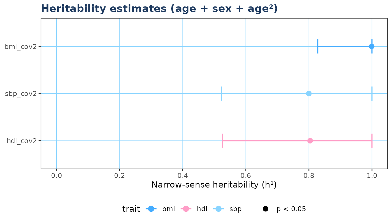
#> 7  bmi_cov2   bmi age+sex_num+age2 240 0.9990 0.1317 0.8251     1    0
#> 8  sbp_cov2   sbp age+sex_num+age2 240 0.8004 0.1401 0.5233     1    0
#> 9  hdl_cov2   hdl age+sex_num+age2 240 0.8052 0.1405 0.5271     1    0
#>   var_covariates sigma2_a sigma2_e
#> 1             NA  0.90510  0.00091
#> 2             NA  0.77409  0.18708
#> 3             NA  0.76987  0.19130
#> 4         0.0209  0.89834  0.00090
#> 5         0.0087  0.76543  0.18952
#> 6         0.0070  0.76629  0.18849
#> 7         0.0307  0.89482  0.00090
#> 8         0.0121  0.76155  0.18992
#> 9         0.0094  0.76945  0.18617
if (requireNamespace("ggplot2", quietly = TRUE)) {
  plot_forest(res, model_filter = "cov2",
              title = "Heritability estimates (age + sex + age\u00b2)")
}